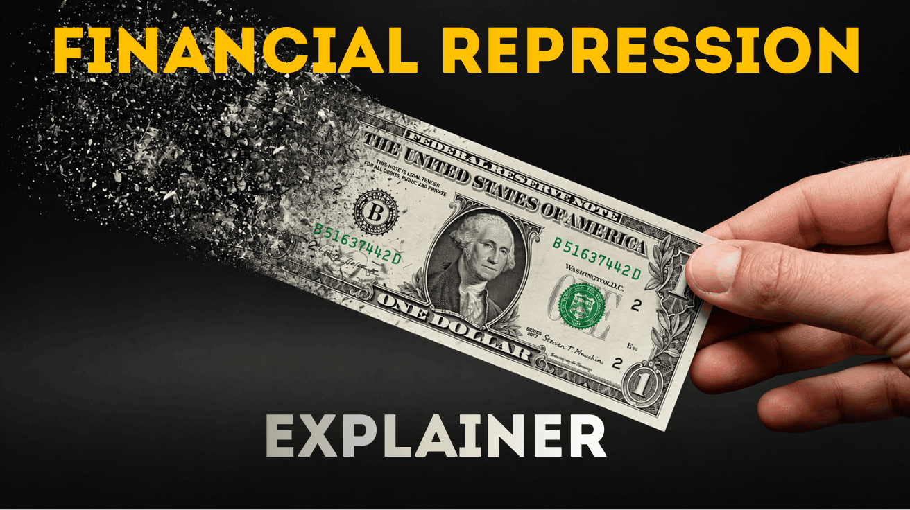
Financial Repression
Financial Repression is a Government Policy Choice that limits what lenders can earn or where savers can put their money, allowing the government or other favored borrowers to borrow more cheaply than they otherwise could. Public authorities can cap interest rates, require financial institutions to hold government debt, or restrict investments that offer savers an alternative. [1][2]
For a family that lends its savings to the government, the consequence can be easy to miss. The Treasury can pay every dollar of principal and interest it promised. Yet if prices rise faster than the interest earned, the family gets back money that buys less than the money it lent. This Inflation erodes the purchasing power of the dollar. Financial repression can keep the lender from earning a return that compensates for that loss. The government, as the borrower, experiences the other side of the same transaction, receiving the benefits. [2][3]
Recession, depression, and financial repression: What’s the difference?
A Recession is a significant decline in economic activity across much of the economy, usually lasting several months. A Depression is an exceptionally severe, often prolonged period of economic weakness. The National Bureau of Economic Research (NBER), which dates U.S. recessions, does not set a numerical threshold at which a recession becomes a depression. [4] Generally though Recessions are 2 or more negative quarters, and Depressions are four or more.
Recession and Depression describe how the economy is doing. Financial Repression describes what public authorities choose to do. Officials can impose a ceiling on bond yields in a growing economy or a shrinking one. They may be trying to finance a war, support an industry, or protect financial stability. Identifying the choice they make does not require assuming that they intended every consequence, including inflation or losses for savers. [1][2]
Why would a government choose Financial Repression?
A government with a large debt has two reasons to want cheaper financing: to leave more room in its budget and to make sure it can find buyers the next time it needs to borrow.
As TPI explains in Ways Out of Debt [5], a country can reduce its debt burden by collecting more revenue, spending less, or growing its economy faster than its debt. But raising taxes or cutting a program requires a visible public choice, and faster economic growth cannot be ordered into existence. Holding borrowing costs down offers a more immediate benefit: the government pays less interest on its debt the next round of borrowing than it otherwise would. [2][5][6]
That next round matters even if the government has stopped adding to its debt. When bonds mature, Treasury must repay their holders. If it replaces those bonds by issuing new ones, it must find lenders willing to accept the new terms. A lower rate does not change the payments promised on an existing fixed-rate bond, but it can reduce the cost of replacing that bond. A government running a deficit also needs buyers for the additional debt it issues. [6] The US is currently running trillion plus deficits annually.
Why would lenders accept less? If lenders/buyers have better alternatives and are free to use them, they may refuse to buy government debt at lower returns. Authorities can change that calculation by requiring banks or pension funds to hold government securities, limiting the movement of savings abroad, or having the central bank buy bonds to defend a ceiling on government borrowing rates. During World War II, the U.S. Treasury and Federal Reserve agreed to hold Treasury rates down to help finance the war. [1][2][7]
There is a political advantage, too. A tax increase shows up on a tax bill. A savings statement has no line showing the interest a family might have earned without a restriction. Economists Carmen Reinhart and M. Belen Sbrancia identify this difference in visibility as one reason governments may find financial repression easier to pursue than an explicit tax increase or spending cut. The government gains some budget room; lenders bear part of the cost through income they never receive. [2]
How Inflation and Financial Repression can work together
The Government owes dollars. The Lender cares what those dollars buy.
A conventional fixed-rate Treasury bond promises interest payments and repayment of principal in dollars. It does not promise how many groceries, gallons of gasoline, or months of rent those dollars will buy. If inflation turns out to be higher than the lender expected, the Treasury can honor the agreement while repaying in dollars that are worth less than the lender anticipated. [2][3][6]
Normally, lenders can adjust. If they expect inflation to continue, they can demand more interest on the next bond or put their money somewhere else. But if policy holds down the yield or restricts their alternatives, it becomes harder to protect their purchasing power. Inflation can reduce the real value of an old debt. Financial repression can help keep the next loan cheap. That combination is especially attractive to a government with substantial debt coming due. [1][2]
This is sometimes described as the dollar “deflating.” The economic terms mean something different. Inflation means the general price level rises and a dollar buys less. Deflation means the general price level falls and a dollar generally buys more. What inflation can reduce is the real burden of a fixed-dollar debt. The number of dollars owed can stay exactly the same. [2][3]
Can keeping government borrowing cheap also contribute to inflation?
Yes, depending on how the policy is carried out. To understand why, separate two decisions often grouped together as “printing money.”
Treasury borrows by selling securities. The Federal Reserve can create bank reserves when it buys an existing security in the open market. The seller gives up the security, the banking system receives reserves, and Treasury still owes the debt. Creating reserves does not automatically put spending money into households’ hands or raise consumer prices. The effect on prices depends in part on how spending changes relative to what the economy can produce. TPI explains the institutional roles in National Debt Components Explained [9]. [3][8][9]
A commitment to cap Treasury yields changes the Fed’s choices. If investors sell bonds, bond prices tend to fall and yields rise. To defend the ceiling, the Fed may have to buy bonds, adding reserves at a time when it would otherwise prefer to restrain credit and inflation. This has happened in the United States. Describing developments after mid-1950, the Federal Reserve Board reported that purchases made to support government securities created bank reserves that “helped to finance the inflation.” [7][10]
The sequence matters. Officials chose to keep government borrowing rates low. Defending that choice contributed to inflationary pressure. That is a documented connection between financial repression and inflation, without claiming that every interest-rate restriction creates inflation or that the Fed caused every postwar price increase. [7][10]
How can the Debt ratio fall without paying down the debt?
The debt-to-GDP ratio compares the dollars the government owes with the dollar value of one year of national output. That second number, nominal GDP (Non Inflation Adjusted), can rise because the country produces more, because the goods and services it produces sell at higher prices, or both. If nominal GDP grows faster than nominal debt, the ratio falls. [6][11]
This is where inflation can make a government’s debt burden look better on paper while a family feels worse off. Existing fixed-dollar obligations do not automatically grow when prices rise. The dollar value of national output can. Holding interest costs down can also slow one source of new borrowing. The government can therefore owe more dollars and still owe less relative to the size of the economy. Meanwhile, the dollars a family saved can buy less at the store. [2][6][11]
A lower ratio is meaningful: it says the debt is smaller relative to national output. It does not establish that the government paid down principal, that the country produced more goods and services, or that households became better off. Nor is a falling ratio guaranteed. If new deficits cause debt to grow faster than nominal GDP, the ratio will rise despite inflation. [6][11] However, if the Debt to GDP ratio is lowered, it can aid in keeping rates lower for Government borrowing, reduce the Debt servicing costs which in turn make more of the Government revenue available to services.
Why this matters now
At the end of fiscal year 2026, U.S. Federal debt held by the public reached ~100% of GDP, according to the Congressional Budget Office (CBO). The amount owed was roughly equal to the value of one year of total U.S. economic output. It was the highest share since 1946. [12]
Debt relative to GDP tells us about the size of the obligation. To see why it matters in the annual budget, ask a different question: For every $100 the federal government collects, how large is its interest bill?
| U.S. fiscal year | Federal net interest outlays | Federal receipts | Net interest per $100 of receipts |
|---|---|---|---|
| 2019 | $375.6 billion | $3,462.2 billion | $10.85 |
| 2026 | $1,051.8 billion | $5,403.3 billion | $19.46 |
Sources: U.S. Treasury, September 2019 Monthly Treasury Statement, Table 9 [13]; Joint Economic Committee, September 2026 Monthly Fiscal Update [14]. TPI calculated the final column using the source figures before display rounding.
Federal net interest went from the equivalent of about one dollar in nine collected to nearly one dollar in five. Meaning the US is paying 20% of all its revenue to essentially credit card interest, that is doing nothing but paying down past borrowing. That does not automatically cut a particular school, road, defense, or retirement program. It means that maintaining the same level of other spending requires more revenue or more borrowing than it would with a smaller interest bill. Borrowing to cover the difference creates another obligation on which future interest may be due. [6][12][13][14] To put it more simply, 1 in 5 of your tax dollars goes to nothing but paying for previous spending.
The pressure can build even when some rates fall. What matters when an old bond matures is how the rate on its replacement compares with the old bond’s rate. A new rate can be below last year’s peak and still be more expensive than the debt coming due. In FY2026, CBO found that more debt and higher long-term rates increased interest costs on publicly held debt, while lower short-term rates offset some of that increase. [12]
Other governments face similar incentives. In October 2026, the International Monetary Fund (IMF) projected global gross government debt at 94.6% of world GDP for the year. It also reported that the average yield on ten-year government bonds across the Group of Seven countries rose by more than one percentage point between February and September 2026. The first figure is a worldwide projection using a broader definition than U.S. federal debt held by the public. The second is an observed change in market borrowing rates. Higher rates reach budgets as governments issue new debt and refinance old obligations. [15][16]
These figures explain why governments want cheaper financing. This doesn’t mean that the United States or any particular country is practicing financial repression today. It may, however to establish that, we need evidence of a policy that held financing costs down or restricted lenders’ choices. [1][2]
What does this mean for the average person?
Start with a bank statement. The nominal balance is the number of dollars in the account. The real balance measures what those dollars can buy. If interest earnings fall short of inflation over the same period (i.e. if inflation growing faster than your money is earning interest), the account can grow in dollars while losing purchasing power. TPI’s Inflation: Measurement Explained [17] explains how price indexes measure that change and why a particular family’s expenses may differ from the average. [3][17]
A saver is asking two different questions:
- Did my return keep up with prices? That tells you whether your savings gained or lost purchasing power.
- Could I have earned more if policy had not restricted my choices? That tells you about the possible cost of financial repression.
A saver can earn more than inflation and still lose potential income because of a restriction. A saver can also fall behind inflation without any such restriction in place. [1][2]
What one dollar bought after World War II
Between March 1946 and March 1947, U.S. consumer prices rose 20.1%. At the end of those twelve months, a dollar held in cash bought about 83 cents’ worth of what it bought at the start. That was a 16.7% loss of purchasing power. The two percentages differ because one measures how far prices rose; the other measures how much an unchanged dollar could buy at the higher prices. [18]
The effect depended on the household. Someone receiving a fixed pension had to stretch the same check further. A worker whose pay kept pace with prices could maintain purchasing power on average, though rent and groceries might follow different paths. A homeowner with a fixed-rate mortgage still owed the same scheduled payment; it became easier to meet if household income rose relative to it. A family could lose purchasing power on its savings while benefiting from having borrowed at a fixed rate. [3][17]
Economists sometimes describe suppressed returns as an implicit tax on savers. No tax bill arrives, and a household’s entire loss of purchasing power does not become a matching receipt at Treasury. The comparison identifies who bears some of the cost of cheaper government financing. TPI explores the analogy in Is Inflation a Stealth Tax? [19]. [2]
Some investors respond by seeking assets they believe will retain their value. Debasement Trade Explained [20] describes that response. A rise in the price of gold, for example, tells us what buyers were willing to pay. By itself, it cannot tell us whether government policy restricted anyone’s return.
World War II: What the government chose and what happened to the debt
During World War II, Americans helped finance the war by buying bonds. For a family participating in a bond drive, that meant giving up spending power then in exchange for dollars later. TPI’s America 250 article, World War II Finance and Mobilization [21], explains how taxes and borrowing funded the war together. Buying a war bond voluntarily was one way to participate. The policy relevant to financial repression was the separate agreement governing the rates Treasury paid. [7][21]
In 1942, Treasury and the Fed agreed on ceilings that included 0.375% on three-month Treasury bills and 2.5% on long-term Treasury securities. To defend those rates, the Fed sometimes had to buy securities. The ceiling on bills ended in 1947, while support for longer-term yields continued. The 1951 Treasury–Federal Reserve Accord restored the Fed’s ability to conduct monetary policy independently of those wartime financing commitments. [7][10]
By then the two institutions faced different problems. Treasury had a large debt to refinance and wanted to preserve inexpensive funding. The Fed wanted the freedom to restrain inflation. TPI’s Fiscal Dominance: Explainer [22] examines that conflict. Financial repression describes controls on financing terms or investment choices. Fiscal dominance describes a condition in which government financing needs constrain monetary policy. [1][7][22]
Treasury and the Fed chose the yield ceilings. The inflationary prices families paid had several causes, including the lifting of wartime price controls, pent-up demand, shortages, and crop conditions. The 83 cent example measures the purchasing power of cash; it is not the realized return on a war bond or Treasury bill. [7][18]
Reducing Debt: The government owed more dollars in 1974 than it owed in 1946
| U.S. fiscal year | Federal debt held by the public | Nominal fiscal-year GDP | Debt held by the public as a share of GDP |
|---|---|---|---|
| 1946 | $241.9 billion | $228.0 billion | 106.1% |
| 1974 | $343.7 billion | $1,482.8 billion | 23.2% |
Source: Office of Management and Budget (OMB), FY2021 Historical Tables, Tables 1.2 and 7.1. Debt is measured at fiscal year-end; GDP covers the fiscal year. Dollar amounts are nominal and rounded for display. [23]
The government owed the public about $102 billion more in 1974 than it did in 1946. Yet its debt fell from 106.1% to 23.2% of GDP because the dollar value of the economy grew far faster than the dollar amount of the debt. The United States did not have to pay down the nominal balance for the burden to decline relative to national output. [6][23]
How Financial Repression reduced the real burden of the debt
During World War II and the postwar years, the Treasury sought low interest rates to finance and refinance government debt. Federal Reserve purchases supporting those rates also contributed to inflation. Describing the inflation after the Korean War began in 1950, the Fed acknowledged that its purchases of government securities “helped to finance the inflation.” These were government financing decisions with consequences for the dollar’s purchasing power. [7][10] www.federalreserve.gov
The government could repay every dollar it promised while returning less purchasing power than it borrowed. Inflation reduced the real value of existing fixed-dollar obligations. When interest failed to keep pace with prices, lenders lost purchasing power even while receiving their scheduled payments. Financial repression helped sustain this outcome by holding borrowing rates below the levels they otherwise would have reached. [2] www.imf.org
The purchasing-power loss was substantial. Earlier in the postwar period, consumer prices rose 20.1% between March 1946 and March 1947, reducing the purchasing power of an unchanged cash balance by approximately 16.7%. That measures the effect of total inflation during that year; a bondholder’s result also depended on interest earned. [18] www.bls.gov
Rising prices also increased GDP measured in current dollars, helping reduce debt relative to the economy. Alongside economic growth and budget surpluses, inflation and restrained interest costs made government debt more manageable. Part of that relief came at the expense of people holding debt whose payments failed to preserve their purchasing power. [2]
How can citizens recognize Financial Repression?
Start with the decision. Who set the rule? What financing terms did it change? What choices did lenders still have? A requirement that banks hold certain government bonds is evidence of directed investment. To estimate its cost, the next question is what those banks could otherwise have earned on investments of comparable risk and maturity. A low Treasury yield by itself answers neither question. [1][2]
Governments also have ordinary ways to manage financing costs. As TPI’s The Treasury Twist Explained [25] illustrates, Treasury can change when its debt comes due. That can change interest costs and refinancing risk without requiring anyone to lend on particular terms.
TPI’s Beautiful Deleveraging [26] considers financial repression alongside choices about taxes, spending, and growth. When a policy promises to make public debt easier to carry, three questions bring the decision back to the citizen:
- Which savers or lenders will earn less or lose an investment choice, and how much is that likely to cost them?
- What public purpose justifies that cost, and how does it compare with the alternatives?
- When the policy ends, will the government be better able to pay its bills at ordinary market rates?
Financial Repression and the American Dream
The American Dream connects work and saving with the opportunity to build a better future: buying a home, paying for education, retiring securely, and helping the next generation get started. Those goals depend on what earnings and savings can buy.
Financial repression can weaken the connection between saving responsibly and getting ahead. When government policy suppresses returns and prices rise faster than interest earned, a savings balance can grow in dollars while losing purchasing power. Families may need to save more or delay their goals to make up the difference. If wages also lag behind inflation, setting aside that additional money becomes harder. [2][3] imf.org
The effects differ across households. People relying on cash savings or fixed payments without inflation adjustments are particularly exposed. A household with a fixed-rate mortgage may benefit if its income rises while its mortgage payment stays unchanged, although other living costs can still increase. The same family can be both a saver and a borrower. [3] imf.org
For the government, restrained interest costs and inflation can make debt more manageable. For savers whose returns are held down, part of that relief comes through earnings they forgo and purchasing power they lose. Economists describe this as an implicit tax on savers, even when no tax rate changes and no separate charge appears on a tax return. [2] imf.org
Financial repression is a policy choice with consequences for opportunity. Citizens should ask whose purchasing power is paying for debt relief, how that burden is shared, and whether the policy preserves families’ ability to build a better future. The bottom line is that unless income is outpacing inflation, or if you are on a fixed income, Financial Repression can make it harder to achieve the American Dream.
Interest costs relative to federal receipts
TPI calculated net interest per $100 of receipts by dividing full-year federal net interest outlays by full-year federal receipts and multiplying by 100. FY2019 uses Treasury’s September 2019 statement; FY2026 uses the Joint Economic Committee’s September 2026 update. Calculations use the source figures before display rounding. $10.85 and $19.46 per $100 compare two budget flows. They are not shares of total spending, do not include principal repayments, and do not mean receipts are earmarked for interest. [13][14]
CBO also reports net interest on the public debt, a distinct measure. Its analysis explains why a larger debt balance and different movements in short- and long-term rates mattered in FY2026. The comparison table uses the budget category net interest outlays consistently in both years. [12][13][14]
Household purchasing power and the debt ratio measure different things
For the cash example, TPI used BLS’s reported 20.1% rise in the U.S. all-items Consumer Price Index from March 1946 to March 1947. Purchasing power retained was 1 ÷ 1.201 = 0.8326; purchasing power lost was 1 − 0.8326 ≈ 16.7%. The calculation assumes an unchanged cash balance earning no interest. [18]
The historical debt table uses nominal fiscal-year GDP, not the Consumer Price Index. It compares debt with the dollar value of domestic production. The one-year consumer price increase is not a measure of inflation’s contribution to the 1946–1974 decline in debt relative to GDP. The household loss on a fixed-dollar payment and the reduction in the real burden of that same payment are two sides of one transaction; they should not be added together. [2][11][18][23]
Reconciling the 117.5% figure in an earlier TPI article
The historical table in TPI’s Ways Out of Debt gives 117.5% as its 1946 starting point and approximately 23% as its 1974 endpoint. Its cited sources suggest a mismatch of years and debt definitions. [5]
The earlier article’s seventh reference contains a gross-debt table showing 117.5% at the 1945 boundary. The FY2012 OMB tables reproduce the figure: $260.123 billion of FY1945 gross federal debt ÷ approximately $221.4 billion of nominal fiscal-year GDP × 100 = 117.49%, or 117.5%. The next row in that edition reports 121.7% for FY1946 gross debt. [27][28]
The earlier article’s eighth reference, Acalin and Ball’s 2023 analysis, instead reports 106% in FY1946 and 23% in FY1974 for debt held by the public. The strongest reconstruction is that a 1945 gross-debt figure was paired with a publicly held debt endpoint and labeled 1946. This is an inference from the cited records; the original calculation worksheet was not located. [24][29]
This article uses the same measure at both endpoints. In the FY2021 OMB edition, debt held by the public falls from 106.1% to 23.2%. If the intended measure is instead gross federal debt, which also includes holdings of federal government accounts, the figures from that same edition are 118.9% to 32.6%. Revisions to GDP can change historical ratios even when the debt dollars stay the same. [23][30]
Treasury’s Debt to the Penny [31] begins in 1993. Historical Debt Outstanding [32] covers earlier years. Treasury’s FY1946 report records $269.422 billion outstanding, a different measure from OMB’s $270.991 billion in gross federal debt. Dividing the Treasury amount by OMB’s $228.0 billion of fiscal-year GDP gives 118.2%. Using BEA’s $227.535 billion of calendar-year GDP gives 118.4% and mixes reporting periods. Neither reproduces 117.5% for FY1946. [23][33][34]
Observations, projections, and research estimates
The IMF’s 94.6% figure is its October 2026 projection for the full year and refers to global gross general government debt. It is not directly comparable with U.S. federal debt held by the public. Acalin and Ball’s 74% figure is a modeled alternative outcome for 1974 under specified assumptions. The observed historical figure was approximately 23%. [15][23][24]
References
[1] Jafarov, E., Maino, R., & Pani, M. (2019; revised May 2020). Financial repression is knocking at the door, again. Should we be concerned? IMF Working Paper No. 19/211, pp. 6–7. International Monetary Fund.
[2] Reinhart, C. M., & Sbrancia, M. B. (2015). The liquidation of government debt. IMF Working Paper No. 15/7, especially p. 15. International Monetary Fund.
[3] Oner, C. (2019, July 30). Inflation: Prices on the rise. Finance & Development. International Monetary Fund.
[4] National Bureau of Economic Research. (2025, October 7). Business cycle dating procedure: Frequently asked questions. Business Cycle Dating Committee.
[5] Tax Project Team. (2025, June 14). Ways Out of Debt: US Options for National Debt. Tax Project Institute.
[6] Congressional Budget Office. (2020, March). Federal debt: A primer.
[7] Anbil, S., & Carlson, M. (2019, March 22). The re-emergence of the Federal Reserve funds market in the 1950s. FEDS Notes. Board of Governors of the Federal Reserve System.
[8] Board of Governors of the Federal Reserve System. (2024, July 19). How does the Federal Reserve’s buying and selling of securities relate to the borrowing decisions of the federal government?
[9] Tax Project Team. (2025, October 17). National Debt Components Explained. Tax Project Institute.
[10] Board of Governors of the Federal Reserve System. (1952). Thirty-eighth annual report of the Board of Governors of the Federal Reserve System, covering operations for the year 1951 (pp. 98–99). Federal Reserve Bank of St. Louis archive.
[11] Garcia-Macia, D. (2023). The effects of inflation on public finances. IMF Working Paper No. 23/93. International Monetary Fund.
[12] Congressional Budget Office. (2026, November 9). Monthly budget review: Summary for fiscal year 2026.
[13] U.S. Department of the Treasury, Bureau of the Fiscal Service. (2019). Monthly Treasury statement, September 2019. Table 9.
[14] U.S. Congress, Joint Economic Committee. (2026, October 22). Monthly fiscal update: September 2026. Fiscal-year receipts and outlays by category.
[15] International Monetary Fund. (2026, October). World Economic Outlook database: World profile. General government gross debt as a percentage of GDP; 2026 projection. Retrieved November 9, 2026.
[16] Dabla-Norris, E., & Valdés, R. (2026, October 15). Rising sovereign yields raise the fiscal stakes. International Monetary Fund.
[17] Tax Project Team. (2025, September 7). Inflation: Measurement Explained. Tax Project Institute.
[18] Reed, S. B. (2014, April). One hundred years of price change: The Consumer Price Index and the American inflation experience. Monthly Labor Review. U.S. Bureau of Labor Statistics.
[19] Tax Project Team. (2024, February 12). Is Inflation a Stealth Tax? The Invisible Price Hike. Tax Project Institute.
[20] Tax Project Team. (2025, October 10). Debasement Trade Explained: What you should know. Tax Project Institute.
[21] Tax Project Team. (2026, June 5). World War II Finance and Mobilization. Tax Project Institute.
[22] Tax Project Team. (2026, February 14). Fiscal Dominance: Explainer. Tax Project Institute.
[23] Office of Management and Budget. (2020). Historical tables, budget of the U.S. government, fiscal year 2021. Tables 1.2 and 7.1.
[24] Acalin, J., & Ball, L. (2026). Did the United States really grow out of its World War II debt? American Economic Journal: Macroeconomics, 18(3), 112–135.
[25] Tax Project Team. (2026, September 24). The Treasury Twist Explained: How America Is Trying to Manage the Cost of Its Debt. Tax Project Institute.
[26] Tax Project Team. (2025, October 22). Beautiful Deleveraging: Reducing debt without pain?. Tax Project Institute.
[27] Wikipedia contributors. (n.d.). History of the United States public debt. Retrieved November 9, 2026. Used only to trace the earlier TPI article’s reference; the figures were verified against OMB.
[28] Office of Management and Budget. (2011). Historical tables, budget of the U.S. government, fiscal year 2012. Tables 1.2 and 7.1.
[29] Acalin, J., & Ball, L. (2023, October 30). Reassessing the fall in US public debt after World War II. VoxEU. Centre for Economic Policy Research.
[30] Congressional Budget Office. (2013, August 12). Updated historical budget data following BEA’s recent update of the national income and product accounts.
[31] U.S. Department of the Treasury, Bureau of the Fiscal Service. (n.d.). Debt to the Penny. Fiscal Data. Retrieved November 9, 2026.
[32] U.S. Department of the Treasury, Bureau of the Fiscal Service. (n.d.). Historical Debt Outstanding. Fiscal Data. Retrieved November 9, 2026.
[33] U.S. Department of the Treasury. (1947). Annual report of the Secretary of the Treasury on the state of the finances for the fiscal year ended June 30, 1946. Federal Reserve Bank of St. Louis archive.
[34] U.S. Bureau of Economic Analysis. (2026, September 30). Gross domestic product, annual (GDPA). FRED, Federal Reserve Bank of St. Louis. Current dollars, calendar years; retrieved November 9, 2026.