The Internal Revenue Service (IRS) uses the term Tax Gap to describe the difference between (1) the amount of tax that should be paid under the law for a given year and (2) the amount of tax that is actually paid. The IRS calls the first concept “True Tax Liability.” The Tax Gap is used by the IRS as a compliance measurement, intended to quantify how much legally owed tax is not collected. [1]
The Tax Gap is often discussed as if it were a single, objectively identified pool of “missing money.” It is not. The Tax Gap is an estimate, based on direct and estimated assessments of missing revenue. What can be directly observed at scale is what taxpayers report and what they pay, both on time and later. What cannot be directly observed at scale, and hence estimated, is “True Tax Liability” for every taxpayer absent intensive verification. That distinction matters because the Tax Gap is built by combining observed payment/reporting data with audit programs, statistical inference, and projections. It is a useful tool, but it is not equivalent to a ledger of collectible receivables. [1][4] While it is entirely likely that some of the non directly observed amount is in fact a true liability owed by tax payers, how much of the figure is up for debate.
How the IRS estimates the Tax Gap
The IRS does not produce Tax Gap estimates in real time. The estimates are developed in study windows and released with a time lag, reflecting the time required to assemble data, conduct audit-based measurement programs, and model components that are not fully observable. As a result, “the latest tax gap” should be read as the latest official estimate for a particular tax year or tax-year range, not as a current-year dashboard. [1][2]
This lag structure also means year-to-year changes in the reported tax gap may reflect changes in underlying compliance behavior, but may also reflect changes in measurement methods, audit coverage, data availability, and economic composition. The Government Accounting Office (GAO), understanding the limits of what is directly observable, has emphasized the importance of continued methodological improvement and transparency in how these estimates are constructed. [4]
Headline versus Reality
Increasingly common in current political dialogue, the Tax Gap is used as a fixed accounting number that “we just need to collect.” This article will explain the Tax Gap, and why the “no brainer” misconception that we can “just collect the tax gap” is incomplete and potentially misleading. As an estimate based on non directly observed data, it is best thought of as a conceptual framework useful in discussions of efficiency, and potential opportunity and not as a true accounting liability. Before we try to use it as a metric, it is necessary to understand what the IRS means by the Tax Gap, what portion is expected to be recovered anyway, and where the largest uncertainties and constraints arise.
“Imagine what we could do for people with $7 trillion.”
Rep. Pramila Jayapal (D-WA) [11]
Gross vs Net: IRS “not paid on time” vs. “never paid”
The IRS reports the tax gap in two related forms:
Gross Tax Gap: the amount of tax liability that is not paid voluntarily and on time. [1]
Net Tax Gap: the portion of the Gross Tax Gap that the IRS projects will remain unpaid after accounting for what is eventually paid through late payments and enforcement. [2]
The difference between the two is critical. It is the IRS’s estimate of the amount that will be recovered after the deadline through enforcement and other late payments. [2] For Tax Year 2022, the IRS estimated:
Gross Tax Gap: $696 billion
Net Tax Gap: $606 billion
Enforced and Other Late payments delta: $90 billion [2]
This Gross-to-Net adjustment is the first major “Headline vs Reality” issue. Public discussion often treats the gross number as if it were the amount available to be collected with additional enforcement. The IRS’s own framework explicitly says otherwise: a portion is expected to arrive later, and a large residual is expected not to arrive. [2]
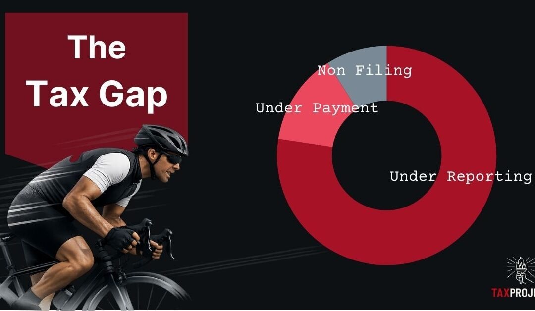
The Tax Gap Components
To understand where the Tax Gap comes from and why it is not simply a matter of “trying harder” the IRS decomposes the Gross Tax Gap into three categories:
Non Filing: required returns not filed.
Under Reporting: returns filed but the Tax liability is understated.
Under Payment: returns filed with correct reported liability, but taxes not paid in full on time. [2]
A Treasury Financial Report excerpt summarizing the Tax Year 2022 projections reports the gross gap as $696.0B, comprised of Non Filing ($63.0B), Under Reporting ($539.0B), and Under Payment ($94.0B) (See Figure 1). [3]
These categories represent distinct levels of observability (and hence reliability), liability from an accounting perspective, and they behave differently with respect to enforcement effort often rising significantly the more you try to collect.
Figure 1 The Tax Gap Source: IRS 2022
Non Filing: a detection problem before a collections problem
Non Filing is frequently discussed as if it were merely a matter of pursuing known delinquencies. In practice, Non Filing is often a detection and identification problem. When a person’s income and activity are captured through strong third-party reporting (for example, routine wage reporting), Non Filing is more readily discoverable. Where reporting is limited or activities are less legible to the system, like small and independent businesses, discovery becomes more resource-intensive and uncertain.
Under Reporting: the largest category and the least directly observable
Under Reporting is the largest component of the Tax Gap, and it is also the most dependent on estimation. Under Reporting spans a wide range of situations: simple misstatements, ambiguous interpretations, valuation disputes, and complex structures. [3][4]
Because “true liability” is not directly observable for most underreporting cases, the IRS uses audit-based programs and statistical methods to estimate the magnitude of underreporting and then adjusts for noncompliance that audits are expected to miss (“undetected” noncompliance). The GAO has examined these methods and urged continued steps to strengthen and improve Tax Gap estimation. [4]
This is one of the central reasons the tax gap is not identical to a known pool of collectible balances. A portion of the underreporting estimate is an inference about what is not seen, not a list of identified cases of actual liability awaiting collection.
Underpayment: where collectability constraints are unavoidable
Underpayment is closest to what the public imagines as “money owed but not paid.” It refers to taxes reported on returns that are not fully paid on time. [2] This category highlights the most basic constraint on “just collect it”: assessments and enforcement actions do not guarantee collection, particularly where taxpayers lack the money (liquidity or solvency) to pay.
Figure 2 Source: GAO
Measured versus Estimated
The Tax Gap combines observed data with inferred quantities.
On the observed side, the government can directly measure:
What is paid on time
What is paid late
What is collected through enforcement [1][2]
On the inferred side, the government must estimate true liability, especially for Under Reporting, by combining audit results, third-party reporting, and statistical adjustments. [4] The IRS also notes that estimates for more recent tax years require greater reliance on forecasts for eventual late and enforced payments because fewer years of post-filing payment history are available. [2]
This is why the Tax Gap should be read with two simultaneous interpretations:
It is an important conceptual compliance benchmark to identify opportunities.
It is not a fully observed accounting liability, fully collectible stock of “missed revenue.”
Once that is understood, the “no brainer” claim begins to look less like a plan and more like a slogan.
International comparisons challenges
Most countries have some Tax Gap in their collections. Seemingly this would be a straight forward way to check the effectiveness of Government collection efforts. However, Tax gap comparisons across countries are frequently apples-to-oranges, for a structural reason: jurisdictions do not necessarily measure the same types/concepts.
A common example is comparing a whole-system compliance estimate to a single-tax gap such as a Value Added Tax (VAT) gap. The European Commission’s VAT Gap is explicitly about VAT, not about the full tax system. [5] Different tax mixes, different reporting regimes, and different denominators further complicate comparisons.
This does not mean international comparisons are impossible; it means they require careful alignment. Like-with-like comparisons (VAT-to-VAT, income-tax-to-income-tax, or genuinely harmonized “percent of theoretical liability” metrics) are informative. Casual rankings built from mismatched definitions are not. [5]
Enforcement Economics: Diminishing Returns
The political shorthand that “enforcement pays for itself” is not inherently wrong; targeted enforcement initiatives can yield substantial revenue. The problem is treating a high marginal return as a constant that can be scaled to close the entire gap.
Treasury Secretary Jacob Lew was quoted in 2013 saying IRS enforcement spending yields $6 for every $1 spent. [6] Whether that ratio is accurate for particular initiatives at particular times, it does not follow that the same ratio holds as a general average across a large-scale enforcement expansion aimed at the full tax gap.
Tax Collection in terms of effort is much like cycling. The amount of effort used while you are going slow is easy, and as you gain speed the amount of effort, and resistance due to wind increases. Each increase is a leap in effort requiring exponentially more effort with each leap. Such is Tax Collection, as collection efforts extend into the long tail—smaller balances, weaker ability to pay, more complicated circumstances collection can become progressively more expensive per dollar recovered. This is a practical constraint that no amount of rhetoric can repeal. In fact, the Congressional Budget Office (CBO) models this into their estimates as the effort increases, the return in revenue drops the more you attempt to collect.
“Thus, in CBO’s estimates, the ROI drops by 10 percent for every 10 percent increase in spending for enforcement and related activities increases”
Congressional Budget Office [7]
CBO explicitly models diminishing returns in enforcement funding. In discussing how changes in IRS funding affect revenues, CBO states that ROI declines as spending for enforcement and related activities increases, providing a rule-of-thumb: ROI drops by 10 percent for every 10 percent increase in enforcement and related spending over baseline. [7]
This modeling choice captures a basic reality: the easiest dollars to collect are collected first. As enforcement expands, agencies move from high-yield opportunities (clear mismatches, strong evidence, high collectability) toward lower-yield opportunities (complex cases, ambiguous positions, weaker collectability, higher dispute and administrative costs). A reasonable way to visualize this is an “enforcement yield curve” where the marginal revenue per enforcement dollar declines as enforcement scales, eventually approaching a low-return tail. (See Figure 3)
The IRS’s own net tax gap concept implicitly reflects this kind of asymptote. Even after late payments and enforcement, the IRS projects a substantial residual remains unpaid. [2]
Figure 3
Biden-era IRS Funding Push
The Inflation Reduction Act provided a major multi-year increase in IRS funding. The public debate often framed this as a means to substantially reduce the Tax Gap, sometimes implying that large sums could be recovered through enforcement and modernization. [8]
In February 2024, Treasury stated that the IRA’s IRS investments would increase revenue by as much as $561 billion over 2024-2034 and cited IRS analysis supporting higher revenue projections than earlier estimates. [8][9] CBO’s general approach, however, is to treat enforcement returns as diminishing and to score them conservatively relative to more optimistic agency scenarios. [7]
The practical interpretation is not that one side is necessarily acting in bad faith. It is that “closing the Tax Gap” is not a mechanical exercise where spending scales linearly into revenue. It is a system where observability limits, administrative capacity, disputes, collectability, and behavioral response create declining marginal returns.
Second & Third Order Effects: avoidance and adaptation
Enforcement is not conducted in a vacuum. When enforcement intensity increases, taxpayers respond. Some responses are lawful, changes in timing, restructuring entities, choosing different tax treatments. Others are unlawful, substitution into less observable forms of evasion. Still others show up as real resource costs—higher compliance spending, higher administrative burden, and greater dispute resolution costs.
These behavioral adaptations are a second reason why the “6:1” ROI cannot be treated as a scalable constant. The more the system stresses a particular enforcement channel, the more taxpayers have incentives to shift behavior toward channels that are harder to police or more efficient from the taxpayer’s perspective (Costlier for the tax collector). At scale, this can reduce the marginal yield of enforcement and can create frictions that affect future taxable activity at the margin.
Even proponents of increased IRS funding recognized the political and practical risks of broad-based enforcement expansion. Secretary Yellen’s 2022 letter emphasized that audit rates should not increase for taxpayers below $400,000 in income, highlighting that enforcement strategy was constrained by legitimacy and feasibility considerations, not merely budget. [10]
Conclusion: a disciplined way to discuss the tax gap
A serious discussion of the Tax Gap should begin with definitions and measurement, not with slogans.
The Tax Gap measures the difference between estimated true liability and amounts paid. [1]
The gross Tax Gap is not the collectible number; the IRS already accounts for late and enforced payments and still projects a large Net Tax Gap. [2]
The largest component, Under Reporting, is also the least directly observable and most dependent on inference and methodological choices. [4]
International comparisons often fail because they compare different taxes, scopes, and denominators. [5]
Enforcement can raise revenue, but returns decline as enforcement scales, and CBO explicitly models diminishing ROI. [7]
Political soundbites such as “$6 for every $1” should be read as claims about limited, high-yield margins, not as a credible strategy to eliminate the entire tax gap. [6][7]
The appropriate framing is not “ignore enforcement,” but neither is it “enforcement will solve it.” The Tax Gap is best treated as a systems problem: strengthen observability where feasible, reduce needless complexity and ambiguity, modernize administrative capacity, and recognize that the last increments of compliance are costly and behaviorally adaptive. Enforcement remains a tool, but it is not a miracle.
The history of Tariffs is a history of the United States from early trade done by local British and Colonial import/exporters to the uniform standards of the Tariff Act of 1789 introduced by James Madison and advocated and implemented by Alexander Hamilton that became the primary revenue source for the young nation. From Congressional lists and schedules updated every 5-6 years by Congress to the dynamically negotiated agreements done by the Executive branch we have today. From an instrument of revenue to a tool for international trade, geopolitical power, and protection of National interests, Tariffs have been used throughout US History. From the disastrous effects of the Smoot-Hawley act to the triumphs of Post World War II Bretton Woods frameworks leading to our current Global Trade.
The First Congress establishes tariff duties as the primary federal revenue source. Congress sets detailed product-specific rates, leading to centralized customs collection at major ports.Significance
Major source of Revenue for United States
Establishes Congressional Authority over Tariffs
First attempt to standardize and provide uniformity to Tariffs across Colonies
Tariff Act of 1828 – a.k.a. Tariff of Abominations – Protective tariffs aimed at Northern industries cause tensions increasing cost of living in the South, leading to the Nullification Crisis when Vice President John Calhoun anonymously penned the Nullification Doctrine which emphasized a state’s right to reject federal laws within its borders and questioned the constitutionality of taxing imports without the explicit goal of raising revenue. Congress still sets rates but political conflicts highlight tariff complexity.
Significance
Establishes use of Tariffs as a Protectionism mechanism to protect domestic industry.
Establishes Congressional Authority over Tariffs
Created Political tension between the winners and losers of any Tariff policy.
The McKinley Tariff Act of 1890 was a high protective tariff raising rates on many imports. Congress remains central in setting rates, with protectionism as a goal. Introduces role of Executive Branch.
Significance
Introduced the concept of reciprocity, lowering tariffs if other country lowered theirs
Introduced role of Executive Branch to manage reciprocity agreements
Wilson-Gorman Tariff Act of 1894 attempts reduction of rates on imported goods and introduces a federal income tax. The income tax is struck down by the Supreme Court until it was re introduced after the passage of the 16th Amendment in 1913, reinforcing tariffs role as major revenue in early America.
Significance
Reduced tariffs on imported goods, reflecting a shift towards lower tariffs
Introduced the concept of Income taxes to offset lower tariff revenue
Contributed to the debate on protectionism vs. free trade, impacting economic policy and government revenue sources.
Creation of the U.S. Tariff Commission: A bipartisan body established to advise Congress with expertise, marking increasing professionalization in tariff policy.
Significance
Predecessor to the US International Trade Commission (USITC)
Led by Frank Taussig, Harvard Professor
Created as part of the Revenue Act of 1916 which introduced Income Taxes
Replaced ad hoc lobby driven policies with analytic and scientific studies and recommendations
Smoot-Hawley Tariff Act – further high tariff rates designed to help farmers exacerbate international trade tensions and the Great Depression. Congressional tariff-setting continues but criticism grows.
Significance
Started Global Trade War – caused retaliatory tariffs and significantly reduced International trade
Considered to contribute to worsening the Great Depression
Global trade levels dropped roughly 2/3rds from 1929 to 1934
Reciprocal Trade Agreements Act (RTAA): Congress delegates authority to the president to negotiate bilateral trade agreements and adjust tariffs within limits dynamically. Beginning of executive role in tariff management.
Significance
Congressional delegation of bilateral trade agreements to the Executive Branch
Allowed President to negotiate +/- 50% of existing Smoot-Hawley Tariff rates
Set Reciprocity as fundamental to negotiating Tariffs that US tariff cuts only if US got a cut in return
Moved Tariffs from Congressional lists to Executive bargaining
Unconditional Multi Lateral Most Favored Nation (MFN) clauses – if you cut Tariff X every country gets the best rate – default multi lateral
GATT (General Agreement on Tariffs and Trade) created a post World War II pact that set the rules for non-discriminatory, tariff-based trade among market economies.
Significance
Locked in Most Favored Nation non-discrimination (Article I): any tariff cut for one member extends to all.
Created bound tariff schedules (Article II), making cuts durable and harder to reverse.
Ran multilateral “rounds” that progressively lowered global tariffs.
Established early dispute settlement norms and a rules-based trading system.
Laid the institutional foundation for the World Trade Organization (WTO)
IEEPA (International Emergency Economic Powers Act) a 1977 U.S. law that lets the President, after declaring a national emergency tied to a foreign threat, block property and restrict transactions to protect national security, foreign policy, or the economy.
Significance
Requires the President to declare a national emergency about a foreign threat.
Allows assets to be frozen and block or allow specific transactions (through OFAC).
Common used for sanctions to limit trade and finance with certain countries, people, or sectors.
Executive branch must report to Congress, and courts can review.
Modern Trump tariffs: The Executive branch imposes broad tariffs using delegated authority and emergency powers to negotiate reciprocal deals. The deals create leverage for US interests, and represent a shift from multilateral deals to US first agreements.
Significance
Broad Tariffs as a negotiating tool in the strong Executive model of negotiation
Goal to reset trade expectations with partners where free trade is reciprocal
Used in geopolitical great power check to limit economic and military threat of potentially hostile peers
Leveraging Emergency Powers (IEEPA) to act on non trade and economic interests like Border Security, and Fentanyl enforcement.
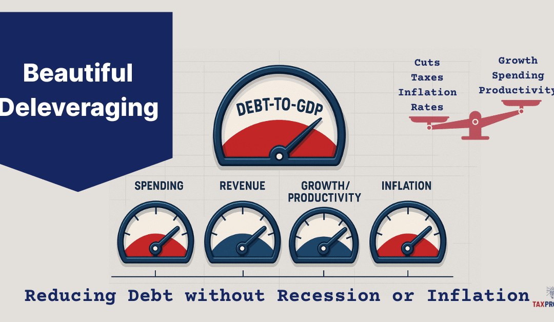
How the U.S. Could Reduce Debt Without Breaking the Economy
The U.S. National Debt just passed $38 trillion according to the US Treasury’s Debt to the Penny. [1][2] Not all debt is bad, but if it gets too large then debt can matter a lot, even those denominated in a fiat currency, because interest costs compound and grow they can crowd out other national priorities. Growing up your parents may have told you that it’s a lot easier to get into something, then to get out. That is especially true for debt, easy to get in, and painful to get out. Now that we have reached the point where interest payments are over $1 trillion annually, the US has crossed into that uncomfortable territory. The real challenge is to bring debt growth under control without causing a recession or a bout of high inflation. Ray Dalio, a billionaire hedge fund manager who has written books on Why Nations Succeed and Fail, and How Countries go Broke, popularized the idea of a “Beautiful Deleveraging” – a balanced, multi-year process that reduces the painful process of deleveraging when lowering debt burdens through a mix of growth, moderate inflation, controlled austerity, and targeted debt adjustments, rather than a painful deleveraging that could lead to recession, extreme reductions in services, tax increases, and austerity measures. [3][4]
This piece frames what a Beautiful Deleveraging could look like for the United States, why it’s hard, the challenges faced, and how policy could balance the Deflationary forces of tightening with the Inflationary tools sometimes used to ease the adjustment—aiming for a soft landing that improves the country’s long-run fiscal and economic health, while minimizing the pain along the way.
Current Status
National Debt: The National Debt stands at just over $38 trillion (gross) with over $30 trillion of which is Debt held by the public. [2]
Deficits: Structural Annual deficits running over $1trillion at around ~6% of GDP. [5][6]
Interest Costs: Net Interest over $1 trillion annually. The Congressional Budget Office (CBO) Long-Term Budget Outlook (March 2025), Net Interest reaches 5.4% of GDP by 2055, up from ~3.2% of GDP around 2025. [7][8] Independent analysis by the Committee for a Responsible Federal Budget (CRFB) highlights a related pressure point: by the 2050s, net interest would consume roughly 28% of federal revenues, absent policy changes. [9]
According to CBO’s latest long-term outlook, by 2055 total Federal outlays (spending) are projected at about 26.6% of GDP, with Net Interest (interest paid on National Debt) near 5.4% of GDP. That means that roughly one-fifth (~20%) of Federal spending will be used to pay interest on the debt. At that scale, interest costs rival or exceed most standalone programs and risk crowding out other priorities if unaddressed. [7][8][9]
What “Beautiful Deleveraging” Means
In Economic terms, Beauty is about reducing debt while avoiding (or at least minimizing) the painful parts of deleveraging and therefore managing that successfully can be Beautiful. Dalio’s Deleveraging framework was originally developed to explain past debt cycles and emphasizes a balanced mix of tools so that the economy can reduce debt without crashing demand and involves these components:
Spending Restraint (public and private demand constraint),
Income growth (real GDP growth),
Debt Restructuring or Terming out (Monetary intervention when necessary), and
A measured amount of Money/Credit creation (Moderating and managing inflation).
These components, when executed with great skill, political courage, and balance, can help the economy grow enough to ease debt ratios while avoiding a deflationary spiral. [3][4]
For a sovereign like the U.S., that balance translates into a policy with credible fiscal consolidation, productivity-oriented growth policies, and a monetary policy that avoids both runaway inflation and hard-landing deflation. Because the U.S. issues debt in its own currency with deep capital markets, it has more room to maneuver than most, but it is not immune to arithmetic: if interest rates (R) run above growth (G) (See our Article on R > G), debt ratios tend to rise unless deficits are reduced. CBO’s long-term projections foresee precisely this pressure in their future outlook. [9]
Pain Points: Why Deleveraging Is Hard
There is a reason it’s hard, in general large broad spending cuts, and more and higher taxes are not popular. While the components and levers are well known, it takes a healthy amount of political courage to propose policies that maybe unpopular, a great deal of skill and coordination to execute these policies, and likely a good amount of luck and good timing for a sustained period likely across several administrations. A deleveraging can proceed along two of these painful paths, spending cuts and tax increases, and each has tangible real-world consequences:
Spending cuts: Less public consumption and investment, fewer or slower growth in transfers, and potentially fewer (e.g. program eliminatinos) or lower service levels (e.g., processing times, enforcement, infrastructure maintenance). In macro terms, cuts are deflationary, they reduce aggregate demand, which can cool inflation but also growth and employment in the short run.
Tax increases: Higher effective tax rates reduce disposable income and/or after-tax returns to investment, is also deflationary. Design matters: broadening the base (fewer exemptions) generally distorts behavior less than steep marginal rate hikes, but either path tightens demand.
Because both mechanisms have a contractionary/deflationary impact and create conditions that can lead to recession, economic hardship, and job loss, a multi-year consolidation approach is part of Dalio’s framework. Instead of a fiscal cliff and extreme austerity based spending cuts; Dalio’s approach phases changes over time; and pairs tighter budgets with growth-friendly policies (innovation, expansion, permitting, skills, productivity increases) that lift the supply side. The goal is to keep nominal GDP growth (real growth + inflation) from collapsing, otherwise debt-to-GDP can rise even while you cut, because the revenue denominator shrinks.
Deleveraging Menu (and Their Trade-offs)
The Tax Project has outlined (See our Article: “Ways Out of Debt”) a non-exhaustive review of policy options to deleverage. Below we provide a summary group them by mechanism. [10]
1) Consolidation via Revenues (Tax Increases)
Summary: Revenue measures (Tax Increases) are deflationary near-term but can be structured to minimize growth drag (e.g., emphasize consumption/external taxes with offsets, or reduce narrow, low-value tax expenditures).
2) Consolidation via Outlays (Spending Cuts)
Summary: Spending cuts can be deflationary; pairing it with supply-side reforms (education/skills, streamlined permitting for productive investment, R&D incentives, labor force productivity growth) can mitigate growth losses and raise potential output over time.
3) Pro-Growth, Supply-Side Reforms (Growth)
Summary: Growth and Supply side reforms (e.g. Productivity, Innovation, Permitting, Energy inputs) that generate real productive growth is the least painful way to lower debt-to-GDP without relying on high inflation.
4) Inflation and Financial Repression (Print Money)
Summary: Modest inflation can ease real debt burdens, part of Dalio’s balance, while managing highly destructive excess inflation. That is why the “beautiful” approach uses only modest inflation alongside real growth, fiscal and monetary management, not inflation as the main lever. [7][9]
The Sooner we Start, the Easier it is
The bottom line is, the longer we wait the harder it gets, the problem will not go away on its own, it only gets worse over time. The 2025 CBO long-term outlook provides a forecast, and it doesn’t paint a great picture:
Debt Outlook: Debt held by the public rises toward 156% of GDP by 2055, under current-law assumptions. [8][11]
Outlays vs Revenues: Outlays (spending) climbs from ~23.7% of GDP (2024) to 26.6% (2055); revenues rise more slowly to 19.3% – expanding an already large and persistent structural gap. [8][12]
Net interest: Reaches 5.4% of GDP by 2055—roughly one-fifth of total federal outlays and around 28% of Federal revenues. [7][8][9]
Those numbers underscore the reason to start now: the later the adjustment, the harder the challenge required to stabilize debt. Conversely, a timely package that the public views as credible and fair can anchor long-term rates lower than otherwise, reducing the interest burden mechanically.
A “Beautiful” U.S. Deleveraging
The Tax Project does not propose or advocate specific policies, however a workable plan using the Dalio Framework would likely include a mix of the following components aimed to stabilize debt-to-GDP within a decade and then bend it downward while sustaining growth and guarding against excessive inflation relapse. A balanced approach:
A multi-year fiscal framework enacted up front allowing for a ordered and measured deleveraging.
Credible guardrails: Deficit targets linked to the cycle; a primary-balance path that improves gradually, with automatic triggers to correct slippage.
Composition: Roughly balanced between base-broadening revenues and spending growth moderation in the largest programs (phased in).
Quality: Protect high-return public investment; target lower-value spending and tax expenditures first.
Administration: Resource the revenue authority to improve compliance; align incentives and simplify.
A growth package to offset the deflationary impulse.
Supply-side reforms with high ROI: energy and infrastructure permitting; skilled immigration; workforce skills; competition policy that fosters innovation and productivity tools.
Private-sector: Reduce regulatory frictions that impede capex expenditures in goods and critical infrastructure.
Monetary-Fiscal Coordination in the background—not Fiscal Dominance.
Monetary-Fiscal Coordination: The Federal Reserve keeps inflation expectations anchored; it does not finance deficits but it can smooth the adjustment by responding to the real economy and anchoring medium-term inflation near target. Over time, a credible Fiscal policy promoting growth helps bring Rates (R) down toward Growth (G), easing the arithmetic. [7][9]
Contingency tools (use sparingly)
“Terming out” Treasury debt Lock in more fixed, long-term loans and rely a bit less on short-term IOUs. Why it helps: If rates rise, less of the debt has to be refinanced right away, so interest costs don’t spike as fast. If the term premium is reasonable and the Fed is in an accommodative stance, shorter term lower rate treasuries maybe attractive to reduce Net Interest expenses.
Targeted restructuring (not the federal debt—specific borrower groups) Adjust terms for groups where relief prevents bigger damage (e.g., income-based student loan payments, disaster-area mortgage deferrals). Why it helps: Stops small problems from snowballing into defaults and job losses while the government tightens its own budget.
This mix qualifies as “beautiful” by balanacing inflationary and deflationary elements. It shares the burden across levers; it avoids hard financial shocks; it relies primarily on real growth + structural balance rather than high inflation or sudden austerity. Done credibly, long-term rates fall relative to a laissez-faire (do nothing) approach, lowering interest costs directly and via lower risk premia. The country benefits both intermediate (by not inducing a recession and harsh economic measures), and long term freeing up revenue to more productive uses than Debt payments, and supporting growth.
Managing the Macro Balance: Deflation vs Inflation
All this sounds good, but the practical art is to offset deflationary consolidation with pro-growth supply measures, not with high inflation. Consider the balancing act between these different variables:
Consolidation (deflationary): Fiscal discipline reduces demand, manages structural gaps, good for taming inflation; risky for growth if overdone or badly timed.
Growth Reforms (disinflationary over time): Expand supply, lower structural inflation pressure; raise real GDP and productivity, improving the debt to GDP ratio.
Monetary Stance: Should keep inflation expectations managed; if growth softens too much, gradual monetary easing is available if inflation is on target.
Inflation temptation: Modest inflation can reduce some of the burden mechanically, but leaning on inflation as the adjustment tool can backfire if markets demand higher interest rate (term) premiums; nominal rates can rise more than inflation, worsening R > G and Net interest. CBO’s baseline already shows interest outlays rising markedly even without an inflationary strategy. [7][9]
A “Beautiful Deleveraging“ aims too creates a “soft landing” keeping nominal GDP growth positive, inflation expectations managed, and real growth strong enough that debt-to-GDP falls without creating undue Economic hardships. Managing each of these variables with the often blunt tools available, many of which don’t manifest for months, or years is quite the magic trick, requiring patience, skill, and acumen.
Risks and Pitfalls
The road ahead can be bumpy and full of challenges, managing the risks is key to a successful deleveraging. Here are some areas that can derail a “Beautiful Deleveraging.”
Front-loaded austerity that slams demand into a downturn or recession; a gradual path anchored by rules and automatic stabilizers is safer and creates less hardships. It means that we will endure less pain over a longer period. Some may want to rip the band aid off and take the measures all at once.
Policy whiplash (frequent reversals) that destroys credibility and raises risk premia (higher Interest rates); stable consistent policies beat one-off “grand bargains” and political vacillations.
Over-reliance on rosy outlooks; plans should make conservative growth assumptions, and reasonable baselines.
“Kicking the can” down the road with laissez-faire policies until interest dominates the budget, leaving painful, crisis-style adjustments as the only option is the biggest of all the Risks. CBO’s outlooks illustrates how waiting raises the eventual cost, and negative consequences. [7][8][9]
Is it Worth it?
On the surface, that’s an easy question, however the answer may pit generations against each other each with their own point of view and different perspectives. Current generations at or near retirement who may not see the worst effects of a laissez-faire policy may see the risk of recession, and cut backs in service as an unacceptable change to their Social Contract which they may have worked a lifetime under a set of expectations that they counted on. Younger generations, may see it as generational theft, placing an undue burden on them for debt they had little or no part in creating. Both are valid perspectives, however, the long term effects of a “Beautiful Deleveraging” will deliver these positive durable payoffs for the Country:
Out of Doom Loop: High debt is a trap, as out of control interest expenses rise, debt grows and the gap between revenue and debt rises in a self reinforcing doom loop. Breaking that loop is key to a healthy economy.
Lower Interest burden: As debt drops, so does Net Interest expenses. Instead of crowding out other expenses, revenue is freed up to other National Priorities (e.g. Healthcare, Education, Infrastructure, Social Services, Surplus, Sovereign Wealth). [7][9]
Greater Macro resilience: With manageable debt exogenic shocks, pandemics, wars, financial events, give the Government financial space to manage these events without taking on negative levels of debt.
Higher Trend growth: When consolidation is paired with genuine productivity reforms, lower debt ratios are correlated with higher growth, supporting living standards and the tax base. [14][15][16]
Summary
A “Beautiful Deleveraging” is but one way to approach the intractable problem of high debt. It represents a reasonable approach that balances near term realities with long term impacts. Our choices now will define the America of the future, and the quality of life younger Americans will have and future generations will inherit. Will it be painless? Probably not, it will likely require some sacrifice and discipline. The challenge wasn’t created in a short period, and it won’t be solved in a short period. Is it achievable? If we face the truth with candor about trade-offs, accept phased steps that the public deems fair, and have a bias toward investments that raise long-term productive capacity, than it is possible. The biggest question is the will of the American people. That, more than any single policy, will determine our future. At the Tax Project we will always bet on informed Citizens making the best choices for America – we will always bet on America. That defines the essence of a “Beautiful Deleveraging.” [3][4][10]
Citations
[1] U.S. Department of the Treasury, America’s Finance Guide: National Debt (accessed Oct. 2025): “The federal government currently has $37.98 trillion in federal debt.” (fiscaldata.treasury.gov)
[2] Joint Economic Committee (JEC) Debt Dashboard (as of Oct. 3, 2025): Gross debt ~$37.85T; public ~$30.28T; intragovernmental ~$7.57T. (jec.senate.gov)
[3] Ray Dalio, What Is a “Beautiful Deleveraging?” (video explainer). (youtube.com)
[4] Ray Dalio, short-form clip on “beautiful deleveraging.” (youtube.com)
[5] Reuters coverage of CBO near-term deficit path (FY2024-2025). (reuters.com)
[6] Associated Press summary of CBO’s 10-year outlook (debt +$23.9T over decade; drivers). (apnews.com)
[7] Congressional Budget Office, The Long-Term Budget Outlook: 2025 to 2055—headline results: net interest 5.4% of GDP by 2055; outlays path. (cbo.gov)
[8] Peter G. Peterson Foundation, summary of the 2025 Long-Term Outlook: outlays to 26.6% of GDP; interest path and historical context. (pgpf.org)
[9] Committee for a Responsible Federal Budget (CRFB), analysis of CBO 2025 outlook: interest consumes ~28% of revenues by 2055; R > G later in the horizon. (crfb.org)
[10] Tax Project Institute, Ways Out of Debt: US Options for National Debt (June 14, 2025). (taxproject.org)
[11] Reuters recap of CBO long-term debt ratio (public debt ~156% of GDP by 2055). (reuters.com)
[12] CBO, Budget and Economic Outlook: 2025 to 2035 (context for near-term path). (cbo.gov)
[15] Cecchetti, S. G., Mohanty, M. S., & Zampolli, F. (2011). The Real Effects of Debt (BIS Working Paper No. 352). Bank for International Settlements.
[16] Eberhardt, M., & Presbitero, A. F. (2015). Public debt and growth: Heterogeneity and non-linearity. Journal of International Economics, 97(1), 45-58.
Confused about the National Debt, why you hear so many different numbers, and what they mean. Here’s a plain English explainer to help you make sense of it all. The National Debt is the total amount the U.S. Federal government owes to its creditors. It does NOT include the Debt held by State and Local Governments. Think of the National Debt as the running total of past annual deficits (when the government spends more than it collects in taxes and other income) minus any surpluses (when it collects more than it spends). The debt grows when there’s a deficit and shrinks—at least relatively—when there’s a surplus or when growth/inflation outpace new borrowing. [1][5]
Terms you should know:
DEFICIT: A deficit is a one-year budget shortfall (this year’s shortfall, which can occur every fiscal year).
NATIONAL DEBT: The debt is a accumulated total of all Deficits minus any Surpluses (the total outstanding IOUs accumulated over time).
Figure 1 Historical Federal Budget Deficits and Surpluses Source: OMB
The U.S. Treasury’s Debt to the Penny website publishes the official daily total and its two big parts (explained below). You can look up yesterday’s number, last month’s, or data back to 1993. [2]
When people talk about the “National Debt,” they often mean one of three closely related figures:
Debt held by the public This is U.S. Treasury securities (Bills, Notes, Bonds, TIPS, etc.) held outside federal government accounts—by households, businesses, pension funds, mutual funds, state and local governments, foreign investors, and the Federal Reserve (America’s central bank). It’s the broadest “market” concept and is the figure economists often use when comparing debt to the size of the economy (debt-to-GDP). [3][4]
Treasury defines it as “all federal debt held by individuals, corporations, state or local governments, Federal Reserve Banks, foreign governments, and other entities outside the United States Government.” [3]
Intragovernmental holdings These are Treasuries held within the federal government – mainly trust funds such as Social Security and Medicare. When these programs run surpluses, they invest in special Treasury securities; when they run cash shortfalls, Treasury redeems those securities to pay benefits, and the government borrows from the public if needed. [4][1]
Total Public Debt Outstanding This is simply the addition of (1) Debt held by the public + (2) Intragovernmental holdings. This is the top-line number on Debt to the Penny. [2][4]
Total Public Debt Outstanding = Debt held by the public + Intragovernmental holdings
Why the distinctions matter:
Debt held by the public is what markets price and what drives interest costs the government pays to outside holders (including the Federal Reserve).
Intragovernmental debt reflects promises among parts of the federal government; it affects future cash needs but doesn’t have the same market dynamics.
Total Public Debt Outstanding is the full legal amount subject to the debt limit (with a few technical exclusions), which matters for statutory debt-limit debates. [4][5] When there are discussion in Congress about the Debt ceiling this is the number discussed.
How deficits add to the National Debt
Each fiscal year, Congress sets taxes and spending. If outlays (spending) exceed receipts (revenue), the government runs a deficit and must borrow by issuing new Treasury securities. Those new securities add to Debt held by the public, and thus to the total debt. The Congressional Budget Office (CBO) publishes baselines and explains the arithmetic and risks of rising Net interest (what the government pays in interest). In 2024, Net Interest on the Debt alone was over $1 Trillion, making it the 3rd largest budget item, larger than National Defense. [5][7][18][22]
In years with a surplus, Treasury can redeem (pay down) outstanding securities or reduce the need to issue new ones—slowing debt growth. But because recent years have seen persistent deficits, the debt has generally climbed. [22]
“Debt to the Penny”
For the Official US National Debt numbers, you can go straight to Treasury’s Debt to the Pennypage. On the site you can:
See today’s total (updated daily except during weekends and holidays) and the split between debt held by the public and intragovernmental holdings.
Download historical CSVs to chart the series yourself.
Check big shifts around tax dates, debt-limit suspensions, or major fiscal packages. [2][15]
Who does what: Role of Treasury vs. the Federal Reserve
The U.S. Treasury (through the Bureau of the Fiscal Service and the Office of Debt Management) issues Treasury bills, notes, and bonds to finance the government at the lowest cost over time. It auctions securities on a regular calendar and redeems them at maturity. Treasury also manages cash (the Treasury General Account at the Fed) to pay the government’s bills. [4][2]
The Federal Reserve (the “Fed”) is the central bank. It does not set taxes or spending and does not decide how much debt the government issues. The Fed’s role here is monetary policy: it influences interest rates and financial conditions. The Fed has a dual mandate to maintain stable prices (control inflation), and manage Employment (manage environment to keep unemployment low). It buys and sells Treasuries only in the secondary market (from dealers), not directly from the Treasury, to maintain its independence and implement policy. [6]
“The Fed does not purchase new Treasury securities directly from the U.S. Treasury, and purchases…from the public are not a means of financing the federal deficit.” [6]
The New York Fed executes these operations for the System Open Market Account (SOMA), the consolidated portfolio of Treasuries and other securities the Fed holds. [12]
What is Quantitative Easing (QE)?
Quantitative easing (QE) is a policy the Fed uses in severe downturns or when short-term interest rates are already near zero. When the Fed is using QE, the Fed buys longer-term securities, such as Treasuries and agency mortgage-backed securities, to push down longer-term interest rates and support the economy. The Fed conducted several large purchase programs after the 2008 Financial Crisis and again during 2020-21 COVID Pandemic. [8][21][14]
Mechanically, when the Fed buys a Treasury, it pays by crediting banks’ reserve accounts at the Fed. That swaps a Treasury security held by the public for a bank reserve (a deposit at the Fed). Crucially, this transaction does not change the total amount of Treasury debt outstanding—it changes who holds it (more at the Fed, less in private hands). [10][6]
“When the Federal Reserve adds reserves…by buying Treasury securities…This process converts Treasury securities held by the public into reserves…[and] does not affect the amount of outstanding Treasury debt.” [10]
Federal Reserve Balance Sheet
Does QE “add to the National Debt”?
No. QE doesn’t authorize or cause Treasury to borrow more or add to the Debt. The deficit determines how much debt Treasury must issue. QE affects yields and liquidity by changing the composition of holders (more at the Fed/SOMA, fewer in private portfolios), not the quantity of debt the government has issued. The Fed repeatedly emphasizes it does not buy securities directly from Treasury or to finance deficits. [6][7][9] (Federal Reserve)
QE can, however, indirectly affect the budget over time through interest rates (lower yields can reduce Treasury’s borrowing costs; the reverse is true when QT—quantitative tightening—lets the portfolio roll off and rates are higher). Several primers walk through these channels. [17][18][7]
How interest flows work when the Fed holds Treasuries
Here’s the accounting workflow in plain English:
Treasury pays interest on all outstanding Treasuries—whether they’re held by a pension fund, a foreign central bank, or the Federal Reserve. That shows up in the budget as Net interest outlays (spending). [18]
When the Fed holds Treasuries (in SOMA), the interest it receives becomes part of the Fed’s net income.
After covering its expenses, the Fed historically remits (gives back) its profits to the Treasury (these are “remittances”). In years when those profits are large, Treasury effectively gets back a chunk of the interest it paid—reducing the government’s overall cost ex post (after the fact). [9][20]
In times (like 2023-25) when the Fed’s interest expenses (mainly interest it pays banks on reserve balances and reverse repos) are greater than its interest income the Fed stops remitting, records a “deferred asset” (an IOU to itself), and resumes remittances only after it returns to positive net income. That deferred asset does not require taxpayer funding; it’s paid down by future Fed profits before any cash flows back to Treasury. [1][5]
“When the Fed’s income exceeds its costs, it sends the excess earnings to the Treasury…When its costs exceed its income, it creates a ‘deferred asset’…and resumes sending remittances after that is paid down.” [1]
Bottom line: whether private investors or the Fed hold a given Treasury, Treasury’s legal obligation to pay interest is the same. The difference is that Fed-held interest often returns back to Treasury (when Fed profits are positive), lowering the government’s ultimate net cost over time. [9][20]
Review of National Debt Concepts
Debt grows because of deficits. Congress’s tax and spending choices determine if there will be an annual deficit or surplus; deficits add to debt. Surpluses reduce the debt. [5][22]
Debt has two big parts. Debt held by the public (including the Fed) plus intragovernmental holdings (trust funds) equals Total Public Debt Outstanding. [2][4] (Fiscal Data)
QE doesn’t “create” more Treasury debt. It changes who holds it and influences rates and liquidity; the Fed buys in the secondary market and does not finance deficits. [6][10][7]
Interest flows are circular when the Fed holds Treasuries. Treasury pays interest; the Fed usually remits (returns) net income back to Treasury; during periods of negative net income, remittances pause and a deferred asset records what will be repaid from future profits. [1][5][20]
You can verify every number daily on Treasury’s Debt to the Penny site, and pair it with monthly public debt reports for detail. [2][4]
FAQ and Common Misconceptions
“If the Fed buys Treasuries, isn’t that just ‘printing money’ to fund the government?” No. The Fed buys from dealers in the open market, not from Treasury. Fed purchases swap Treasuries for bank reserves; they don’t change the amount of debt or directly finance the deficit. [6][10][7]
“Doesn’t the debt count everything the government owes, including future Social Security benefits?” The debt is legal obligations already issued (Treasury securities). Future promises (like future benefits) affect the budget and future borrowing, but they aren’t counted as debt until the government issues securities to pay for them. These are called Unfunded Liabilities (See our Article). Check the Debt to the Penny site for what is counted. [2][4][5]
“Why do some charts focus only on debt held by the public?” Because that’s the portion traded in markets, driving interest costs and macro impacts. It’s also the number most used in economic comparisons (for example, debt-to-GDP). [5]
Debt Guru: How to read the daily debt like a pro
Visit Debt to the Penny site and note Total Public Debt Outstanding.
Compare the split between public and intragovernmental. Persistent deficits typically raise the public share over time.
If rates are rising (or have risen), expect net interest in the budget to climb; CBO’s primers explain why interest costs can grow faster than the economy when debt is large. [2][18][22]
If you want more depth on how the Fed runs these operations, the New York Fed’s archive on large-scale asset purchases and the Board’s description of the System Open Market Account are the canonical sources. [8][12]
Putting it all into Context
If you want to understand how big the National Debt is, how it relates to other things like the size of our economy, how the budget deficits and surpluses compare in charts over the years historically and how that impacts the debt in charts, check out that and more in the Tax Project Institute’s Smarter Citizen App (A Free Citizen App, just register – no credit card and you’re in!)
Treasury security: An IOU the U.S. government sells to borrow money (Bills mature in a year or less; Notes in 2–10 years; Bonds in 20–30 years; TIPS are inflation-protected). Holders earn interest and get their principal back at maturity. [3]
Debt held by the public: Treasury IOUs owned by investors outside the federal government, including the Federal Reserve. [3]
Intragovernmental holdings: Treasury IOUs held by government accounts (e.g., Social Security trust funds). [4]
QE (quantitative easing): The Fed’s large purchases of longer-term securities to lower long-term interest rates when the economy needs help and short-term rates are generally already lower. [21][8]
Remittances: Fed profits (if any) sent to Treasury after covering expenses; paused when the Fed’s interest expenses exceed income (recorded as a “deferred asset”). [5][1]
References
[1] Board of Governors of the Federal Reserve System. (2024, July 19). How does the Federal Reserve’s buying and selling of securities relate to the borrowing decisions of the federal government?https://www.federalreserve.gov/ (Federal Reserve)
[2] U.S. Department of the Treasury, Fiscal Data. (n.d.). Debt to the Penny (daily dataset; coverage back to 1993). Retrieved October 16, 2025, from https://fiscaldata.treasury.gov/ (Fiscal Data)
[3] U.S. Department of the Treasury. (n.d.). Public Debt FAQs (definitions of debt held by the public & intragovernmental holdings). Retrieved October 16, 2025, from https://treasurydirect.gov/ (TreasuryDirect)
[4] U.S. Department of the Treasury, Fiscal Data. (n.d.). Monthly Statement of the Public Debt (MSPD) (monthly dataset). Retrieved October 16, 2025, from https://fiscaldata.treasury.gov/ (Fiscal Data)
[8] Board of Governors of the Federal Reserve System. (2025, September 23). Interest on Reserve Balances (IORB): FAQs (includes note that asset purchases convert Treasuries to reserves without changing outstanding Treasury debt). https://www.federalreserve.gov/ (Federal Reserve)
[10] Board of Governors of the Federal Reserve System. (2016, August 25). Is the Federal Reserve “printing money” in order to buy Treasury securities?https://www.federalreserve.gov/ (Federal Reserve)
[12] Board of Governors of the Federal Reserve System. (n.d.). Fed Balance Sheet—Table 1 (popup): U.S. Treasury, General Account (definition of the Treasury General Account). Retrieved October 16, 2025, from https://www.federalreserve.gov/ (Federal Reserve)
[13] Board of Governors of the Federal Reserve System. (n.d.). H.4.1—Factors Affecting Reserve Balances (current and archived releases). Retrieved October 16, 2025, from https://www.federalreserve.gov/ (Federal Reserve)
[14] Federal Reserve Bank of St. Louis (FRED Blog). (2023, November 20). Federal Reserve remittances to the U.S. Treasury.https://fredblog.stlouisfed.org/ (FRED Blog)
[15] Board of Governors of the Federal Reserve System (via FRED). (n.d.). Liabilities & Capital: Earnings Remittances Due to the U.S. Treasury (RESPPLLOPNWW) (weekly series). Retrieved October 16, 2025, from https://fred.stlouisfed.org/series/RESPPLLOPNWW (FRED)
[16] Board of Governors of the Federal Reserve System. (2024, March 26). Federal Reserve Board releases annual audited financial statements (deferred-asset explanation). https://www.federalreserve.gov/ (Federal Reserve)
[17] Anderson, A., Ihrig, J., Kiley, M., & Ochoa, M. (2022, July 15). An Analysis of the Interest Rate Risk of the Federal Reserve’s Balance Sheet (Part 2). Board of Governors of the Federal Reserve System, FEDS Notes. https://www.federalreserve.gov/ (Federal Reserve)
[19] U.S. Department of the Treasury, Fiscal Data. (n.d.). America’s Finance Guide: National Debt (dataset links and coverage notes—e.g., Debt to the Penny since 1993). Retrieved October 16, 2025, from https://fiscaldata.treasury.gov/ (Fiscal Data)
[20] Data.gov (U.S. General Services Administration). (n.d.). Debt to the Penny (dataset catalog entry and composition note). Retrieved October 16, 2025, from https://catalog.data.gov/ (Data.gov)
[22] U.S. Department of the Treasury, Fiscal Data. (n.d.). Historical Debt Outstanding (long-run series). Retrieved October 16, 2025, from https://fiscaldata.treasury.gov/ (Fiscal Data)
When it comes to the Federal budget, several terms are used and it is important to understand what they are in order to know how they are funded, and how they shape the overall Federal budget. So, if you are interested in understanding the Federal budget, understanding these terms is a must. Most federal spending fits into three categories. Understanding how and why these categories work can help you understand the Federal Budget process and what programs keep paying even during funding lapses, why others pause, and where most dollars are actually spent. They can also help you understand what constraints Congress is under, knowing each of these categories will help you understand how little discretion there is in the budget without legal changes. For a high level understanding of these three categories in FY2024: Mandatory Spending programs were a bit over $4.1 trillion (~60%), Discretionary Spending programs about $1.8 trillion (~26%), and Net Interest (i.e. interest paid on the National Debt) about $1.0 trillion (~14%), for roughly $6.8 trillion in total Federal outlays (spending). Net interest is shown as its own category in official presentations. [1][2][3]
What each Category Means
Mandatory Spending: This category of spending, as its name implies, is required by statute (law). Budget items in this category are automatically authorized for funding unless the law is changed. The statute (law) sets which programs are mandatory and the eligibility requirements and formulas for how much is authorized. Mandatory spending was about $4.1T in FY2024—roughly 60% of total outlays. [2][3]
Entitlements: This category is a subset of Mandatory Spending. Entitlements are Mandatory Spending programs that confer a legal right to benefits to citizens, for example: Social Security, Medicare, and Medicaid are Entitlements. Entitlements make up the bulk of Mandatory Spending; Social Security and Medicare alone account for more than half of mandatory outlays. [2]
Net Interest: The interest the U.S. pays on its National Debt. It’s authorized by permanent law (a permanent, indefinite appropriation) [4], which is why many sources describe it as “technically mandatory,” but it is shown as its own category in the budget, separate from both mandatory and discretionary. In FY2024 it was about $1.0 trillion (~14% of total outlays). [1][3]
Discretionary Spending: This is the remaining non-compulsory spending, everything Congress has not defined by statute (law). Short of changing the law on Mandatory Spending programs, this is the part of the budget Congress can adjust annually. Discretionary spending is just over one-quarter of total outlays (~26%). Congress decides discretionary levels each year during the Federal budget process in 12 separate appropriations bills produced by the Appropriations Committees. (See our Article on Federal Budget Process.) [1][5]
Figure 1: Federal Budget Categories FY 2024 Source: CBO
What’s inside each Category
Mandatory Spending
Programs
Description
Entitlement
FY 2024 Budget Amount
% of Total Federal Spending
Social Security (Old-Age, Survivors, and Disability)
Provides benefits to retired workers, the disabled, and their spouses, children, and survivors. Funded by payroll taxes.
Yes
$1.45T
21.4% [2]
Medicare
A federal health insurance program primarily for people age 65 or older and certain younger people with disabilities.
Yes
$0.9T
12.7% [2]
Medicaid and CHIP
A federal-state health care program for low-income and needy individuals, including children, pregnant women, the elderly, and people with disabilities.
Yes
$0.6T
9.1% [2]
Veterans’ disability compensation and pensions
Provides benefits to veterans who have a service-connected disability. Pensions are paid to low-income wartime veterans.
Yes
$0.2T
2.8%
Federal civilian and military retirement
Provides retirement benefits to federal government civilian employees and military personnel, including pensions, disability, and survivor benefits.
No
$0.2T
2.9%
Unemployment Insurance (federal share)
A joint federal-state program that provides temporary, partial wage replacement to unemployed workers.
Yes
$0.03T
0.5%
SNAP and other nutrition programs
Provides benefits to low-income households to supplement their food budgets. Other programs include school lunch, and food assistance for seniors.
The part of tax credits that can be paid as a refund.
Yes
$0.16T
2.4%
Affordable Care Act (a.k.a. Obamacare)
Provides tax credits and other subsidies to help eligible individuals and families afford health insurance.
Yes
$0.11T
1.6%
Farm programs (e.g., crop insurance subsidies)
Provides subsidies and other support to farmers and agricultural producers.
No
$0.03T
0.5%
Other Mandatory Programs
A collection of smaller, non-entitlement mandatory outlays not separately itemized, such as deposit insurance, payments for natural resources, and other government-wide programs.
No
$0.3T
4.1%
Subtotal Mandatory Spending
$4.1T
~60%
Net Interest
Program
Description
FY 2024 Budget Amount
% of Total Federal Spending
Net Interest
Debt Service – Interest payments on US National Debt
$1.0T
~14%
Discretionary Spending
Programs
Description
FY 2024 Budget Amount
% of Total Federal Spending
National Defense
Funds for the Department of Defense (military operations, personnel, weapons procurement, research), and other defense-related activities in other agencies.
$0.9T
~13% [1]
Health and Human Services
Discretionary funds for health research (e.g., NIH), public health, and human service programs, separate from Medicare and Medicaid entitlements.
$0.1T
~2%
Education
Provides funding for federal education initiatives, grants, and programs at all levels.
$0.1T
~1%
Transportation
Supports highway and airport construction, mass transit, and other infrastructure projects (note: highways/aviation have mandatory contract authority, but spend-out is shaped by annual limits).
$0.1T
~1%
Veterans’ Health Care
Funds health care services provided through the Veterans Health Administration (separate from mandatory disability compensation).
$0.1T
~2%
Homeland Security
Funds for agencies responsible for homeland security, including border patrol and immigration enforcement.
$0.06T
~1%
Housing & Urban Development
Public housing, community development, and housing assistance programs.
$0.06T
~1%
Energy & Environment
Department of Energy, Environmental Protection Agency, and other natural resource and environmental programs.
$0.06T
~1%
International Affairs
State Department, USAID, and foreign aid.
$0.06T
~1%
Other Discretionary
Various government agencies and programs, including general government administration, science, and space exploration (e.g., NASA/NSF).
$0.3T
~5%
Subtotal Discretionary
~$1.8T
~26%
Summary
Knowing Federal Budget terms is useful for understanding how and where Federal money is spent. In FY2024 the Federal Government spent ~$6.8 trillion and took in ~$4.9 trillion, with a deficit of ~$1.8 trillion. The majority of the spending goes to Mandatory programs, most of which are Entitlement programs providing services and benefits to citizens. Net interest—about $1.0T—is reported as its own category and paid under permanent law. As the Mandatory components grow, there is less room for Discretionary items that Congress can administer without reductions in mandatory spending, increases in tax revenue, or additional borrowing. When you look at discretionary spending, many people would consider those categories essential – Education, Environment, Transportation, National Defense – core services of government. Understanding these components clarifies the difficult trade-offs between fiscal sustainability and key government services. [1][2][3][4][5]
Citations
[1] Congressional Budget Office (CBO), The Federal Budget in Fiscal Year 2024: Infographic; and Discretionary Spending in FY2024: Infographic (discretionary ≈ $1.8T; composition; total outlays context). [2] CBO, Mandatory Spending in Fiscal Year 2024: An Infographic (mandatory ≈ $4.1T; Social Security + Medicare > half of mandatory). [3] CBO, Monthly Budget Review: Summary for Fiscal Year 2024 (total outlays ≈ $6.8T; net interest ≈ $0.95T, rounded to $1.0T). [4] 31 U.S.C. § 3123, Payment of obligations and interest on the public debt (interest paid under permanent, indefinite appropriation). [5] CBO primers on budget categories and the annual appropriations process (12 appropriations bills produced by the Appropriations Committees).
Tax Project Institute is a fiscally sponsored project of MarinLink, a California non-profit corporation exempt from federal tax under section 501(c)(3) of the Internal Revenue Service #20-0879422.


 9")

 11")